Second Order Analysis Options per Load Case

The standard analysis method in MasterFrame is a 1st order linear elastic analysis. Where elements such as tension only members, no axial force members (📄 Member Attributes) or spring restraints (📄 Nodal Supports) are included in a model the software automatically carries out an iterative analysis process to reflect the presence of these elements or restraints.

The Second order analysis option opens the Analysis Options pane, which opens in the right side of the window. When the pane opens, the software defaults to load case 001 and none of the available options are selected. The initial pane is shown below.

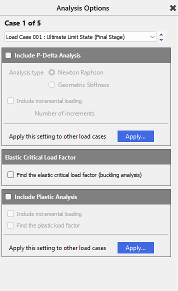
Include P-Delta analysis

This enables a P-Δ analysis to be carried out on specific load cases, to account for the geometric deformation of a structure

The P-Delta analysis utilised in MasterFrame is a P-Δ analysis, which modifies the frame geometry under loading and re-analyses the model in the deflected position. The software carries out an iterative process, carrying out the analysis a number of times, modifying the frame geometry for each iteration, until either an equilibrium condition is reached, or, if equilibrium is not reached, a frame stability warning is given.

Two methods of P-delta analysis are available, the Newton Raphson method or the Geometric Stiffness method.

Analysis Type

Geometric Stiffness method

In the Geometric Stiffness the method, the bending stiffness of the elements in any model are modified to account for the axial force present in the member. Compressive forces will reduce the bending stiffness, while tensile axial forces will increase the element stiffness. In the case of a member which is loaded to its Euler buckling compressive load, the bending stiffness will be reduced to zero. The reference of the geometry remains in its original undeformed configuration. This is know as the total Lagrangian approach.

In the Geometric stiffness method, only two iterations are carried out, the first to calculate the axial force under a linear static analysis, the second iteration to account for the modified member stiffnesses in bending.

Since the geometric method only uses two iterations, it is less computationally demanding that the Newton-Raphson method, so, for larger models, it requires less time to analyse than would be required for the Newton Raphson method. However, with only two iterations, the method takes less account of the geometric deformation of the structure under load. Thus, the Geometric Stiffness method is less suitable for the analysis of structures where the deformation of the structure is significant. As a result, the Geometric Stiffness is less generally applicable than the Newton Raphson method.

Newton-Raphson method

The Newton-Raphson non-linear iterative method carries out a series of analyses, modifying the stiffness matrix of the structure to account for the deformation of the structure from the previous analysis. This is know as the updated Lagrangian approach. At each stage of the analysis, the out-of-balance forces due to the difference in the external and internal model forces is calculated. The process is continued until the out of balance in the external and internal forces is within a prescribed tolerance, within a specified number of iterations.

The process terminates when either (a) The analysis converges to a solution where the out of balance forces are within tolerance, or, (b) The analysis diverges and a solution is not possible. There may be circumstances where out of balance force convergence is difficult, and the software can automatic attempt a deflection based convergence criteria if this option is chosen in the User Defined Non-Linear Convergence Settings in the 'Analysis> Global Analysis Option' screen.

The Newton Raphson method uses the dX, dY and dZ translations of the nodes within a model to assess the deformation of the model geometry in each iteration. This means the internal deformation of the members themselves is not assessed as part of the analysis, unless the member contains intermediate nodes. Intermediate nodes can be added to a member by splitting the member (see Modify Geometry>📄 Splitting Members for details). Alternatively, analytic nodes can be added to a member. Where internal nodes are added to a member, then the deformation of the member is accounted for, to some degree, within the analysis.

In general, the member deformations are of less significance than the nodal deformations of the model. In terms of the member design, in the concrete design additional moments are added as the design stage to account for the internal deformations of the members, while in the steel and timber design, effective lengths and member buckling as accounted for at the design stage.

The Newton-Raphson method would be the most generally applicable type of P-delta analysis.

See User Defined Non-Linear Convergence Settings (📄 Global Analysis Options).

Include Incremental loading

The load is applied in increments and the positions any plastic hinges is determined at each load increment and the positions of any hinges is used in the next step in the loading. This assists in determining which hinges form in which order.

(Find the

Find the Elastic Critical Load factor

Enable the calculation of the elastic critical load factor for specific load cases

The Elastic Critical Load factor option uses a matrix analysis method to identify the lowest buckling mode of the structure. This method is based on the geometric stiffness matrix method, which modifies the standard stiffness matrix to account for the compressive force in an element. Where an element has a compressive force, the bending stiffness of the member is reduced, whereas a tensile force will increase the bending stiffness of a member. For a member loaded to its Euler Critical Buckling load, the Geometric stiffness method (📄 P-delta Analysis) will reduce the bending stiffness of the member to zero.

The Elastic Critical Load factor is the elastic buckling load divided by the axial load on a member. For each individual load case, the axial load on the member is derived from the analysis of the particular load case.

With the Elastic Critical Load option active for a load case, the analysis of that load case will find the load factor at which the analysis no longer has a solution, indicating the structure is no longer stable. An iterative approach is used to find the load factor at which buckling occurs.

The results of the Elastic Critical Buckling analysis are given the Graphical Analysis Outputs, accessed by going to Results>Graphical Analysis Results. The Elastic Buckling factor is reported in the right-hand pane for those load cases where the Elastic Critical Load Factor option was activated.

In the 📄 Graphical Analysis Results, the Elastic Critical Buckling mode shape can also be shown graphically for any load case where the analysis option was active.

The Elastic Critical Buckling Load Factor method identifies the largest factor at which the analysis no longer completes, indicating the system of equations can no longer be solved. This indicates the structure is no longer stable. However, the instability may occur when a single member becomes unstable, or it may indicate the overall structural system has become unstable.

Elastic Critical Buckling Load Factor versus alpha-crit analysis

Both the Eurocode and British Standards provided a method to calculate the factor by which the design load would need to be increased to cause elastic instability in the global frame. In the Eurocode this is the alpha-crit factor, while in the British Standards this was the lambda-crit factor. Both the alpha-crit and lambda-crit calculations are based on the sway buckling mode of the structure, being based on the horizontal deflection under the horizontal design load. The aim of the alpha-crit and lambda-crit methods is to determine the global instability mode of the structure based in the initial elastic stiffness and the lateral deflections of the structure.

In a structure where the global instability is dominant and the whole structure buckles first (often referred to as the Sway Mode), then the Elastic Critical Load factor method would be expected to give a similar Elastic Load factor as the alpha-crit and lambda crit-methods. However, if the buckling of an axially loaded member dominates the analysis and it is this Elastic Critical factor that the Elastic Critical method identifies, then the buckling mode identified will not be that of the global structure and therefore it is highly likely that the Elastic Critical Load factor method will result in a significantly different load factor than would result from the alpha- or lambda-crit methods.

💡

If local member elastic critical buckling load factors is important (non-sway mode), it is necessary to model the member with an appropriate subdivision of analytical members, with a minimum of 3 internal evenly distributed nodes recommended. You can do this using the Modify Geometry> Split Member choosing 4 segments and using the Insert analytical nodes only option.

The Graphical Analysis Output allows the display of the Elastic Critical Buckling Mode shape. This displays the deformed shape of the structure at the point of the elastic critical load. The deflection is normalised (scaled so the maximum value of deflection equals 1), as this is mode shape and not a real world deflection. To determine if the buckling shape is global, it is necessary to review the overall mode shape and make an engineering judgement.

Include Plastic Analysis

Consider the formation of plastic hinges where members have been selected to have one or more plastic hinges

The use of the plastic analysis option means that within the analysis, the software will calculate the formation of plastic hinges at predefined locations. In order for the load case to include plastic analysis this must be turned on for the loading case from 'Analysis> Second Order Analysis Option per case'

💡

Plastic hinges can only be formed when a 'Potential Plastic Hinge' has been placed. These can only be placed at analytical member ends. If intermediate member plastic hinges are required, the member must be split to insert a further analytical node at which to place a potential plastic hinge.📄 Potential Plastic Hinges

The plastic moment capacity used for the hinge is determined as follows

For Class 1 Steel Sections Library 'I' sections or user defined class1 'Built-Up I' sections, the plastic moment capacity is automatically determined an analysis time and is dependent on any co-existing member axial force
For non-dimensioned 'User defined' sections, i.e. where all the basic section properties are specified, the plastic moment value can also be input.
The member attribute 'Moment Limit' 📄 Member Attributes can be used to specify the plastic moment value and where present overrides the above two values.

The plastic hinge will only allow a moment up to and not exceeding the plastic moment at the point of the plastic hinge.

The software uses an iterative approach when using the Plastic analysis. An initial elastic analysis is carried out to determine the point of maximum moment and a plastic hinge applied. The analysis is then re-run and the modified bending moments calculated. Further plastic hinges are determined, if selected and the process repeats until either a solution is found, or sufficient plastic hinges form such that the structure is no longer stable, in which case an analysis warning will be given, identifying the node at which the instability occurs.

The Plastic Analysis is specified on a per load case basis.

The Plastic Analysis includes two options when applying the Plastic Analysis to any load case. These options are: -

Include Incremental loading

Find the plastic load factor

This option calculates the moment at the hinge position at which a hinge would form, compared to the moment at that point in the load case under consideration and takes a ratio of the two moments to return the plastic hinge formation moment as a ratio of the moment due to the load case. A ratio less than 1.0 indicates that the plastic capacity of the member is less than the moment which would occur at that point in the load case under consideration. Where the Load Factor ratio is greater than 1, then the plastic capacity is greater than the moment applied in the load case under consideration.

The plastic load factor is given in the 📄 Graphical Analysis Results. Refer to the Results chapter for further details.

Apply this setting to other Load Cases

To enable the Plastic Analysis to be applied to several load case, rather than having to go load case by load case, clicking on the Apply icon will open the Apply Plastic Analysis Setting Loading Cases pane. This pane is shown below.

To apply the Plastic Load analysis, select the load case in the upper pane. The load case will highlight blue. To multi-select load case, hold the Ctrl key and then click on each required load case in the upper right-hand pane. The load cases can be scrolled using the mouse wheel

In the bottom pane, options are providing to allow the quick selection of load cases. The selection will be shown in the upper pane, with the selected load case highlighted in blue.

Clicking the Apply icon will add all the plastic analysis to the selected load cases.

Clicking Close will close the Apply Plastic Analysis Settings Loading Cases window and go back to the Analysis Options Window.

At the foot of the pane, links are provided to quickly access other menu items. These include the Global Data, including material densities (📄 Member Global Density), 📄 Coefficient of Thermal Expansion and📄 Live Load Reduction, 📄 Load Cases which opens the 📄 Load Combinations menu. The Notional Loads navigates to the horizontal notional load 📄 Notional Horizontal Loading / Equivalent Horizontal Force menu.