MasterFrame FE Analysis: Circular Concrete Tank Setup Tutorial
This tutorial outlines the most efficient method for creating a circular tank structure using rotational copy commands and Finite Element (FE) surfaces, rather than manual grid line generation.
Generating the Tank Geometry
Open MasterSeries: Begin by launching the MasterFrame application.
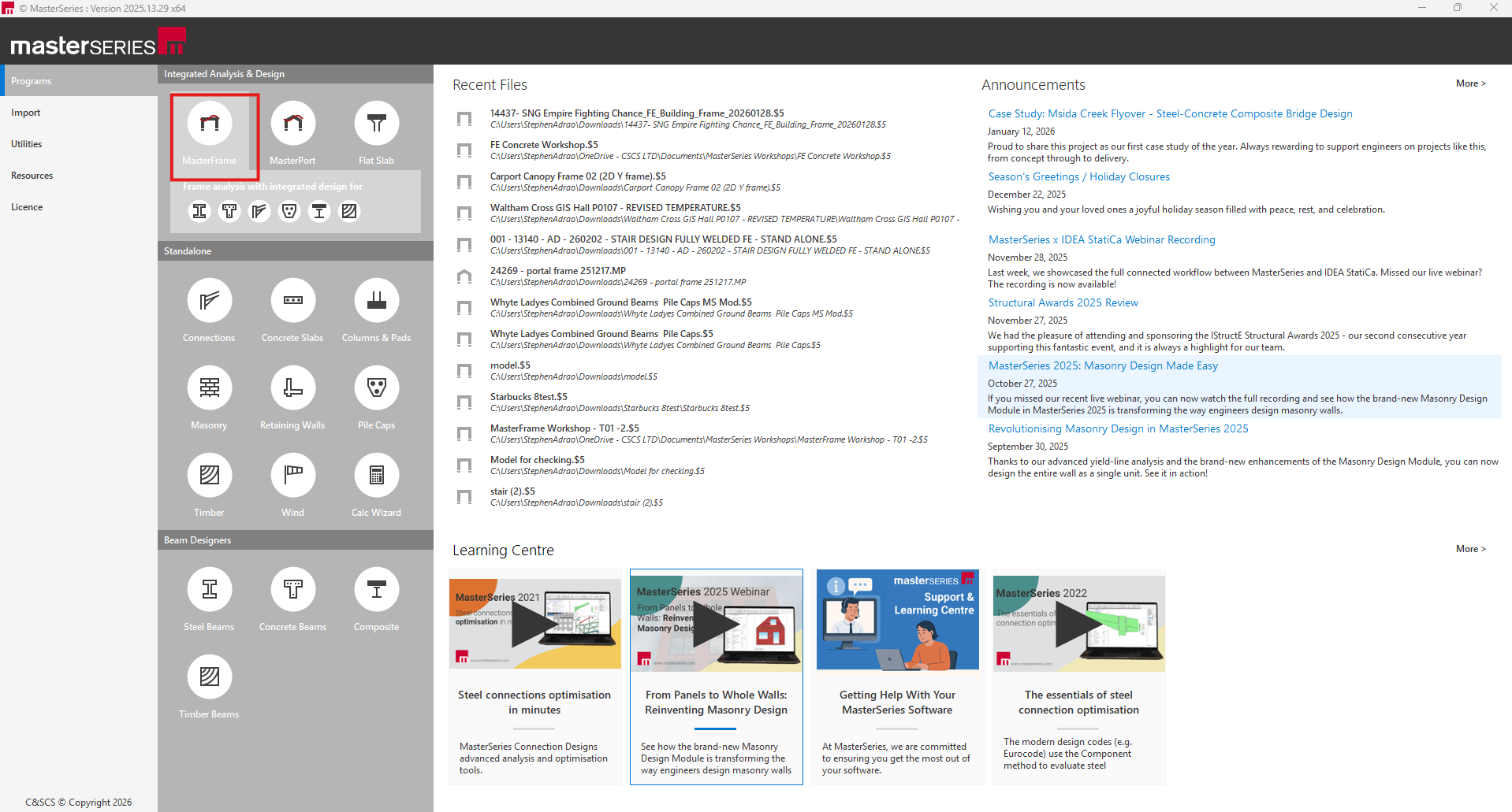
Create a New File: Select the option to create a new file and name it accordingly (e.g., "Circular Concrete Tank").
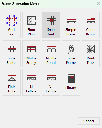
Snap Grid: Ensure the snap grid is selected at the start to assist with initial placement.
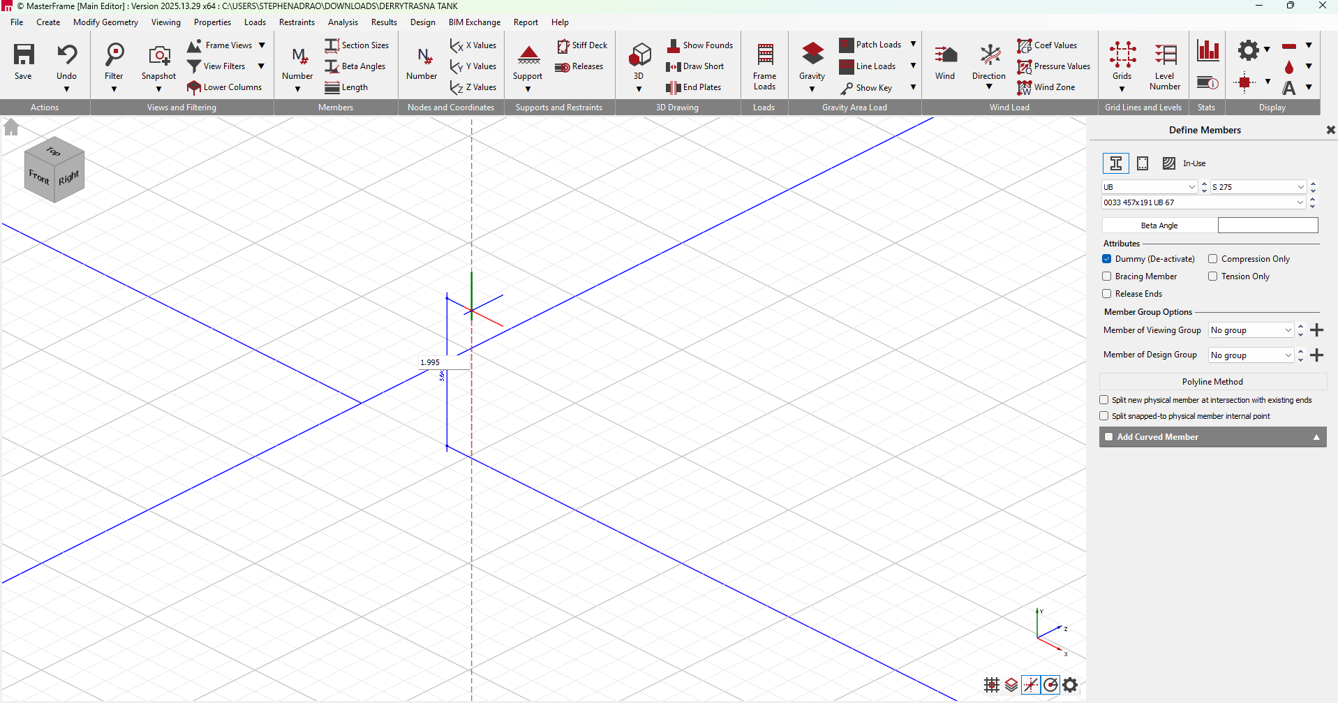
Create a reference member
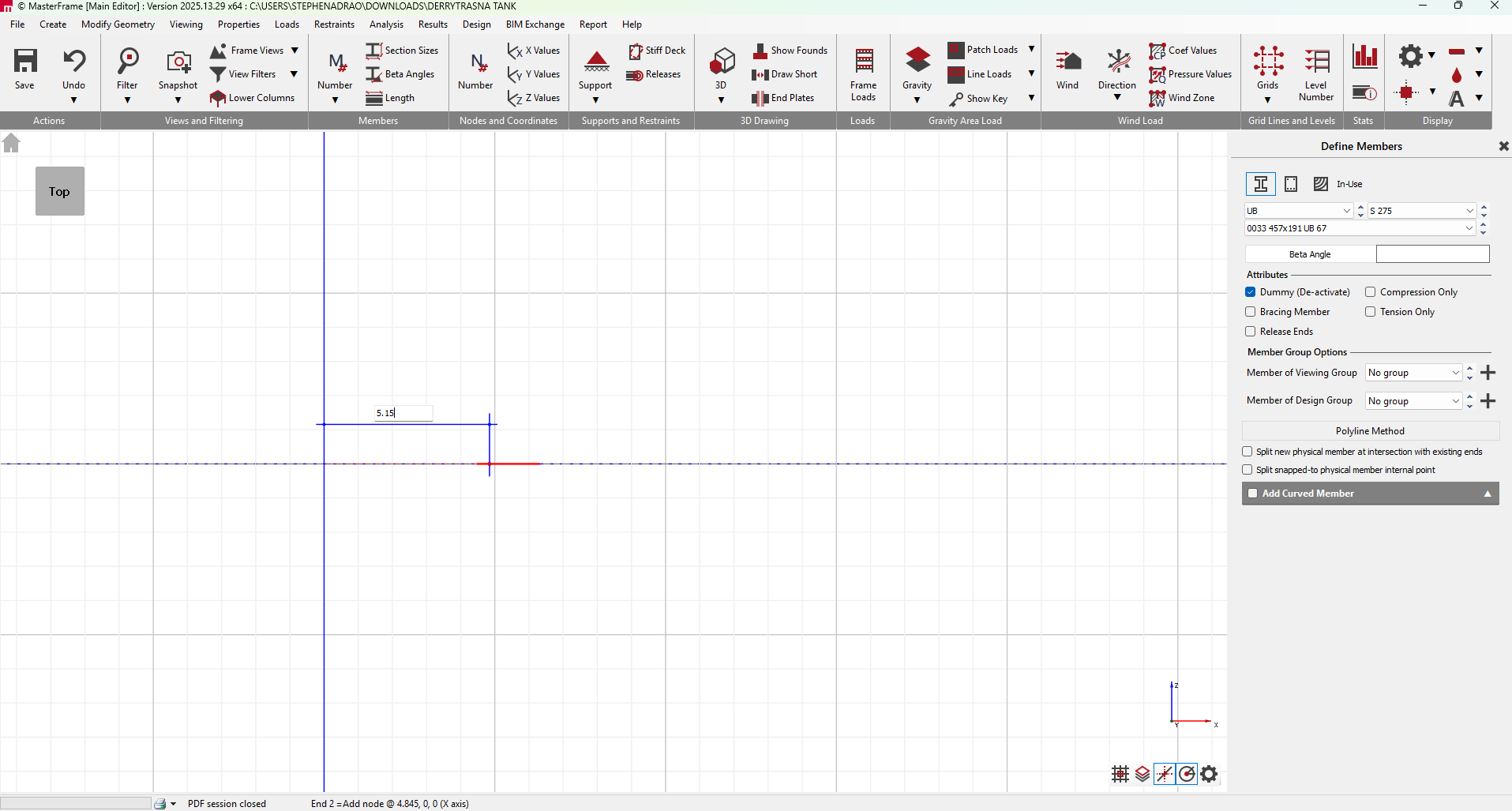
- Go to Create > Add Member.
- Define a "Dummy Member" (this will act as a construction line and will not affect the analysis).
- Select the Top View (
 )
) - Define the Base Node: Start at coordinates 0, 0, 0 (the center of the tank).
- Define the Radius: Draw a member outwards to the tank radius. For example, if the radius is 5.15m, draw to 5.15, 0, 0.
- Define the Wall Height: From the radius point (5.15, 0, 0), draw a vertical member up to the wall height (e.g., 1.955m). This vertical line represents the edge of one segment of your wall.
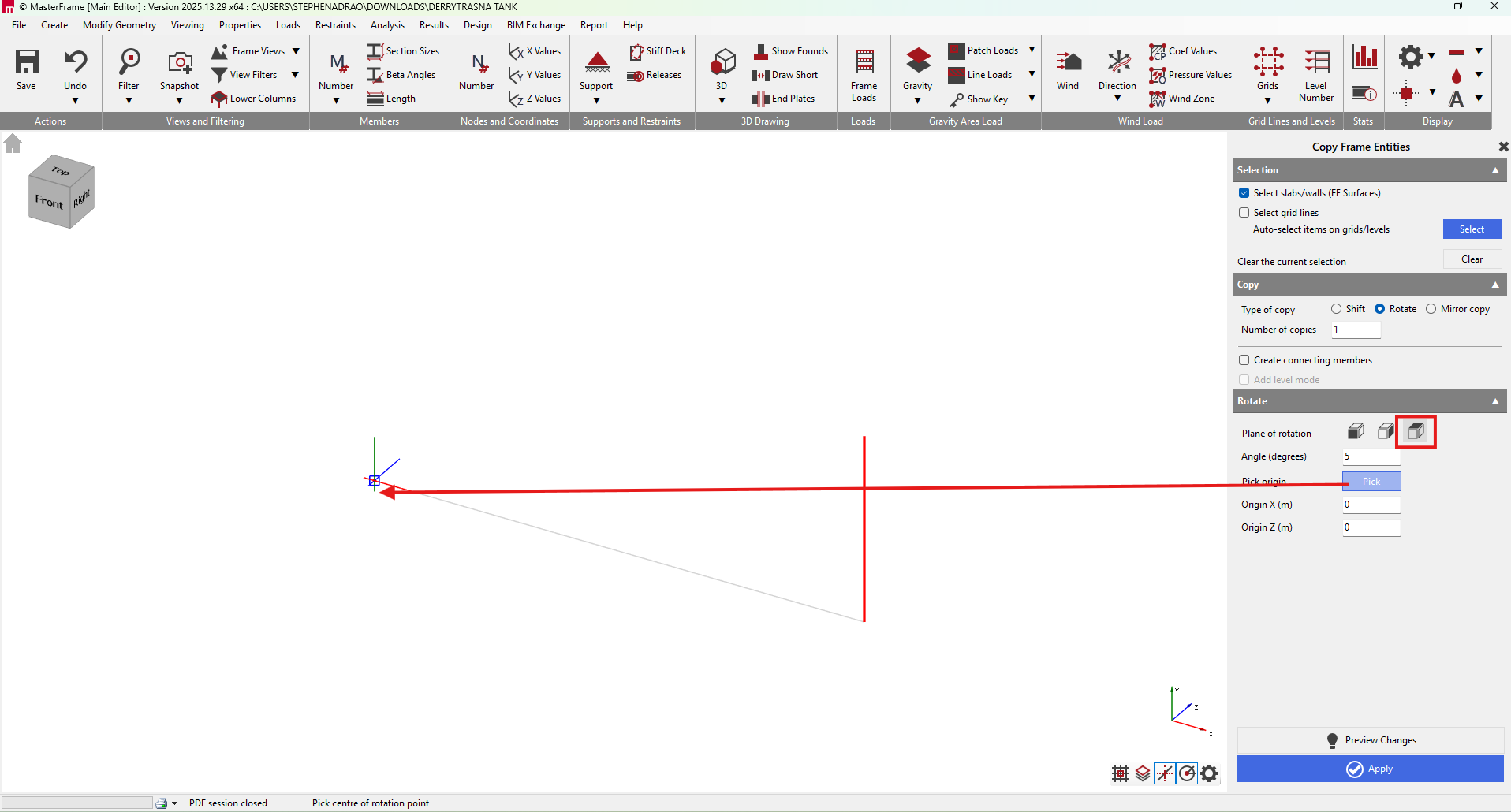
Create the first Segment
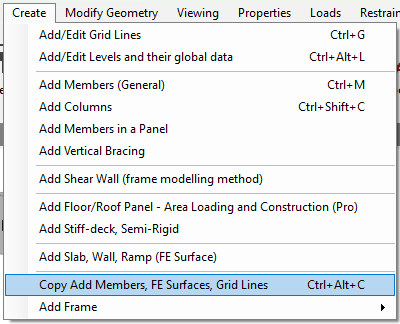
- Go to Create and Copy, Add Members, FE Surface, Grid Lines.
- Use the rotate and copy function to replicate this member.
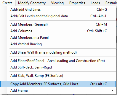
- Set the rotation to 5° increments and generate 1 copy first.
- Select the origin as (0,0) and ensure to connect the members.
- Click Apply.
Defining an FE Surface
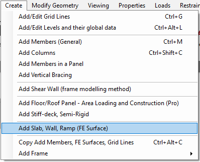
- Add an FE surface using these boundaries by going to Create > Add Slab, Wall, Ramp (FE Surface).
- Select the boundary members of the vertical wall segment to create a valid FE surface
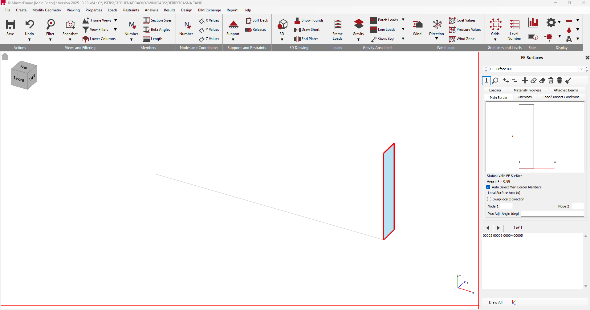
- Go to Material/Thickness and assign a material of 300mm thick concrete. Assign a grade of C35 and ensure you have ticked Codified Materials.
Load Application
Area Loads
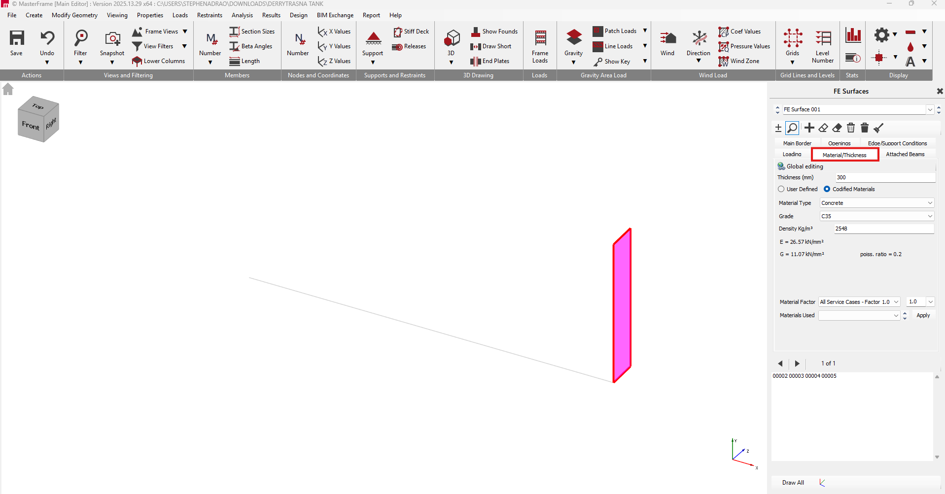
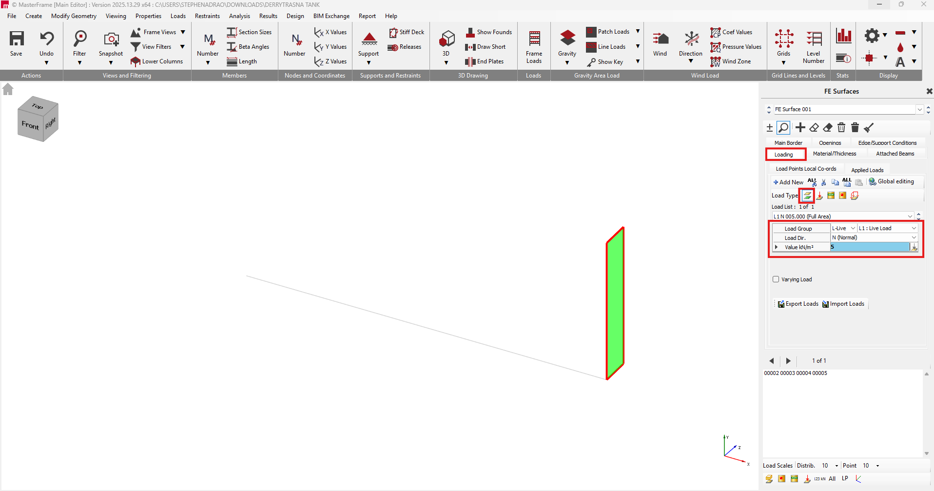
- Go to the Loading tab and apply an Area loading as a Live load at the normal with a 5kn/m3 value.
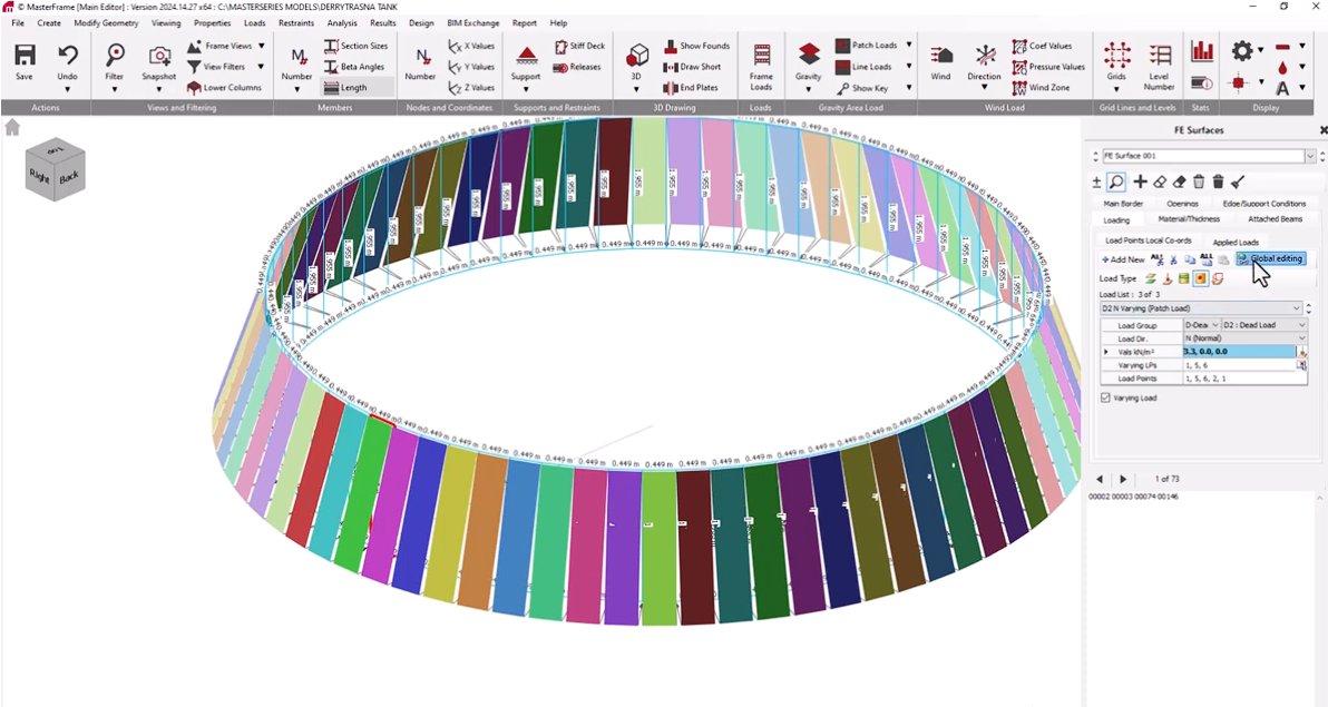
Applying Advanced Patch Loads
Add a new load, we'll be adding a Patch load instead of traditional area loading, this method uses specific coordinates to define load outlines. Create a dead load at the normal with a value of 17.7,0,0kn/m3.
Define Load Points: Create six specific load points to serve as references. After applying the bottom two points, go up 1.805m and then click on the two points at the top to create six points.
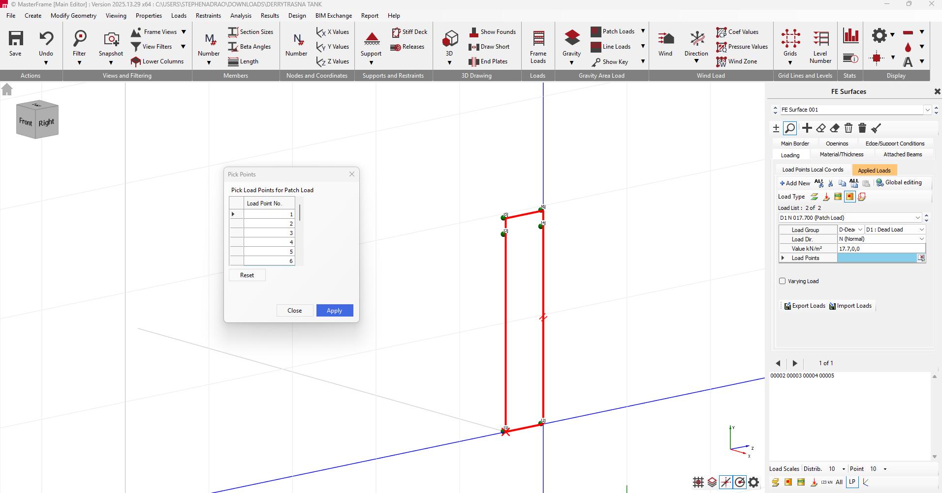
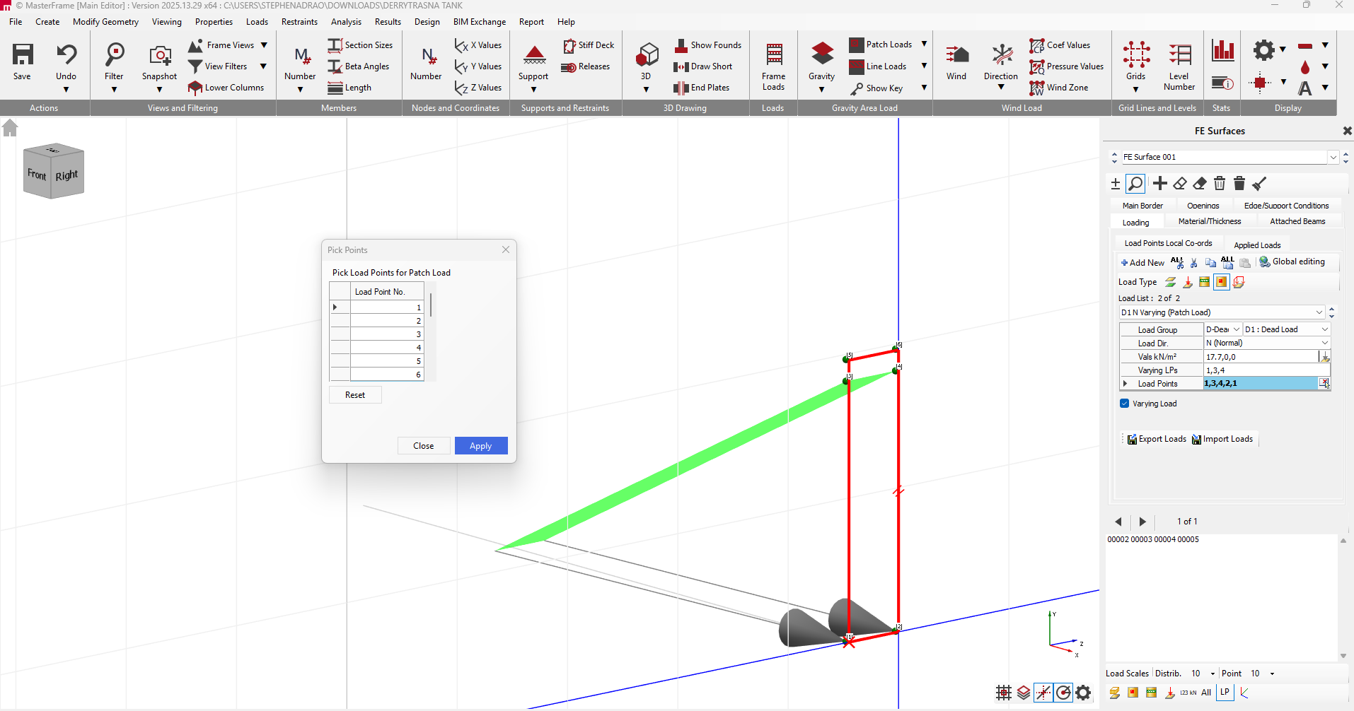
Set Patch Loads: Apply a patch load normal to the surface face. Use a varying load type and reference the previously created load points to define the load's outline (e.g., points 1, 3, 4, 2, 1).
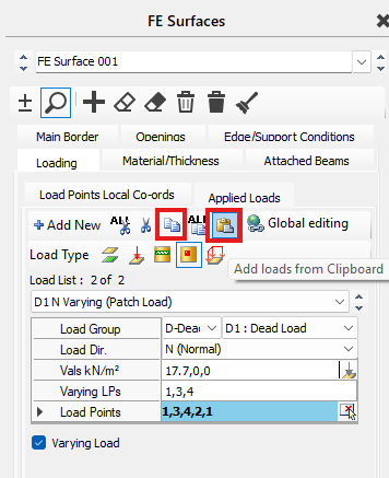
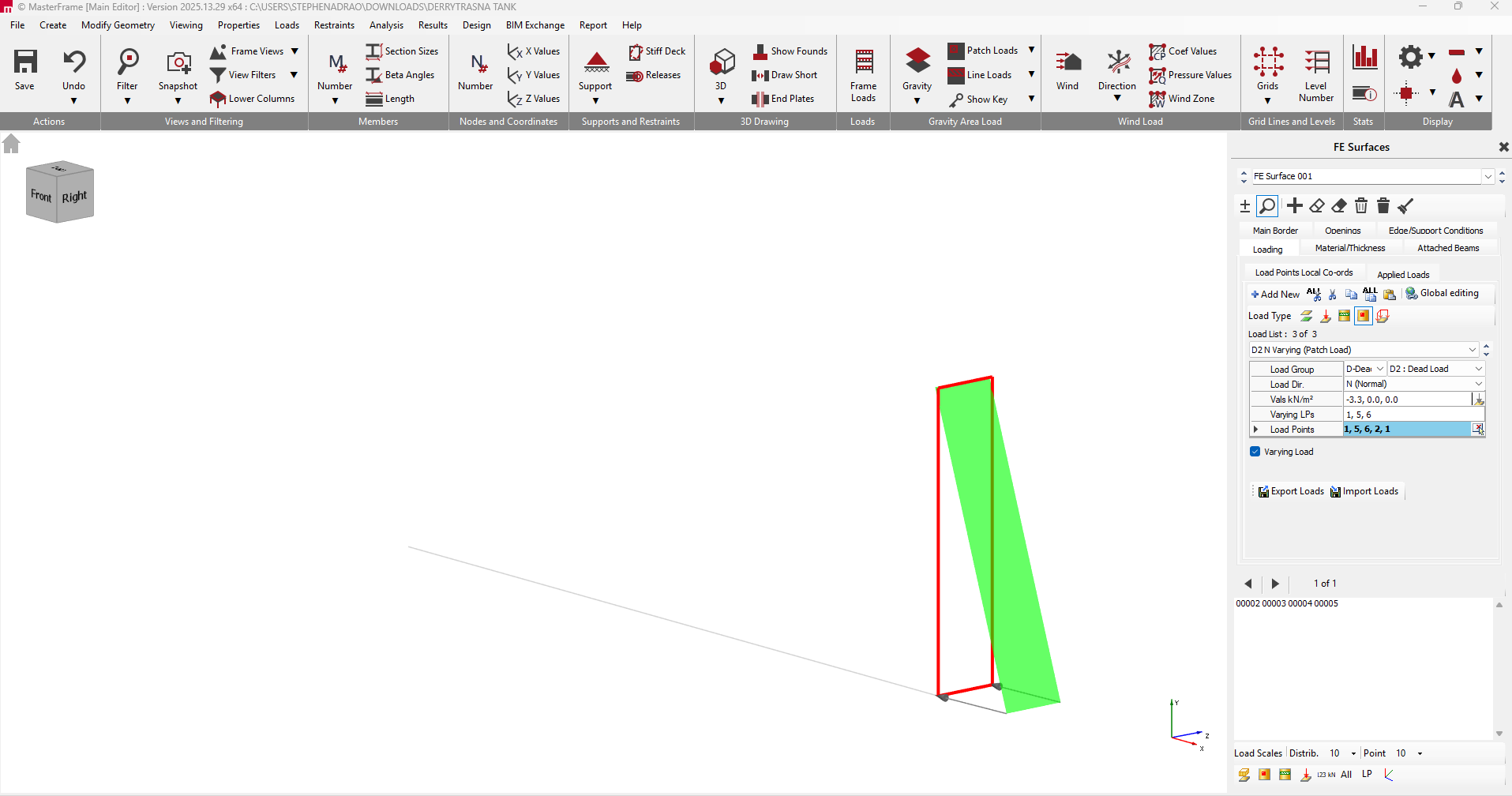
Replicate Loads: Once defined for one surface, copy and paste these loads.
Locate the load you just created, change the load to D2, change the direction to -3.3 and the varying loads/load points to 5 and 6.
Future Amendments: A primary benefit of using load points is the ability to easily adjust water levels later by simply amending the load points rather than reconfiguring the entire mesh.
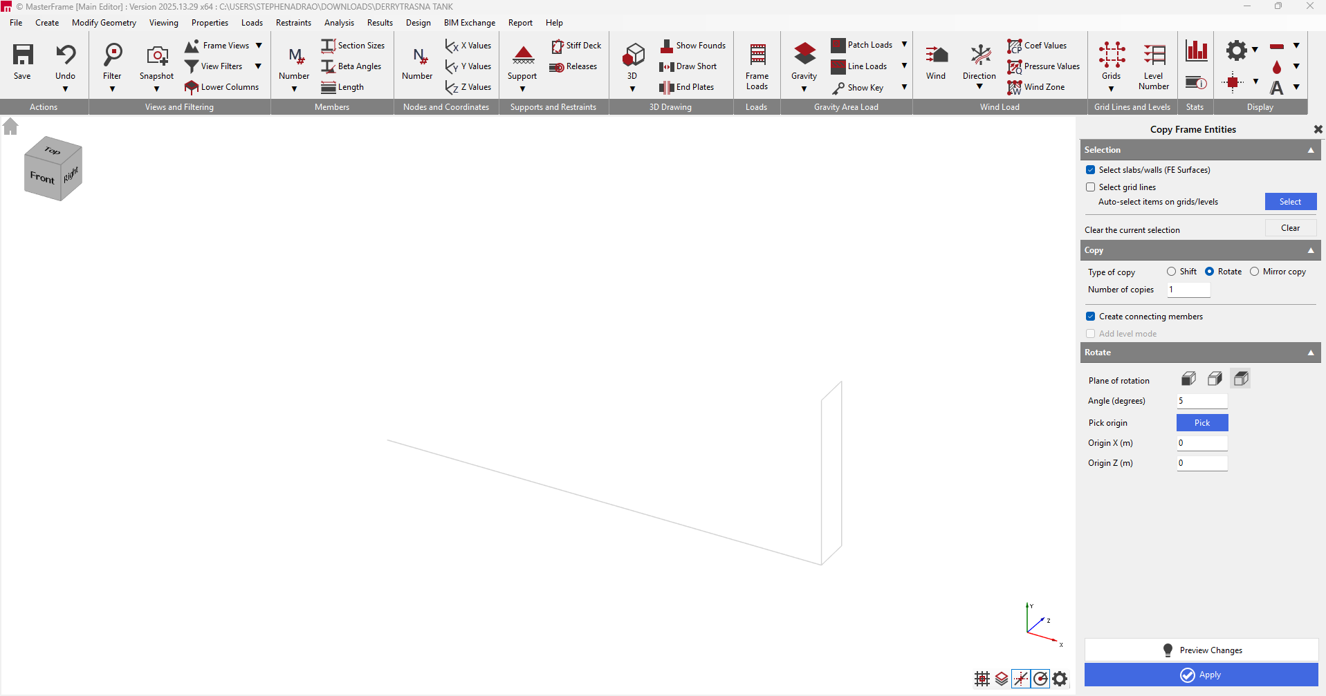
Creating the Circle Tank Geometry
We will now create the circle geometry, go to Create and then Copy Add Members, FE Surface, Gridlines.
Select the surface, create 71 copies with a rotation of 5 degrees with the origin at (0,0).
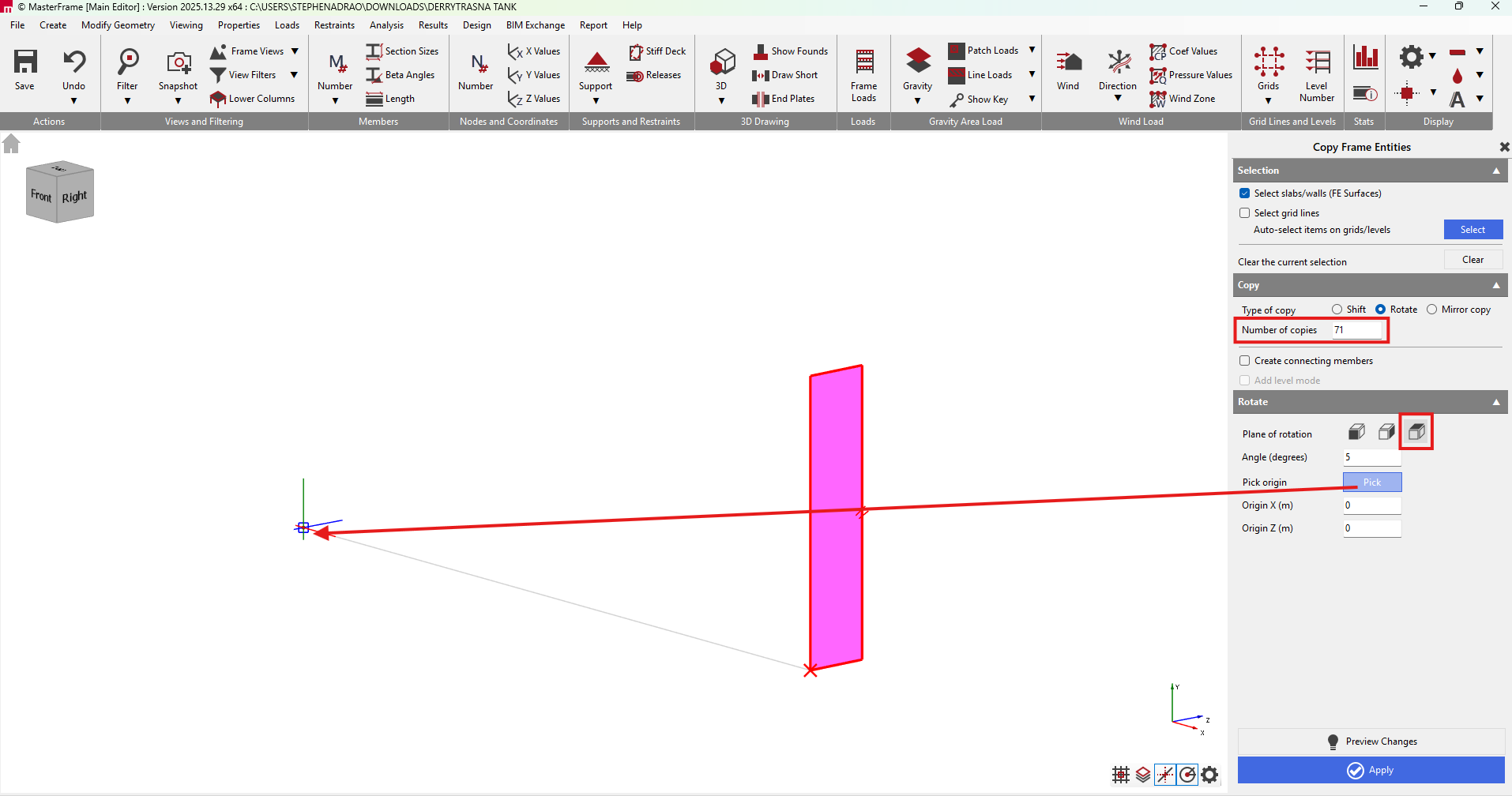
Click on Apply.
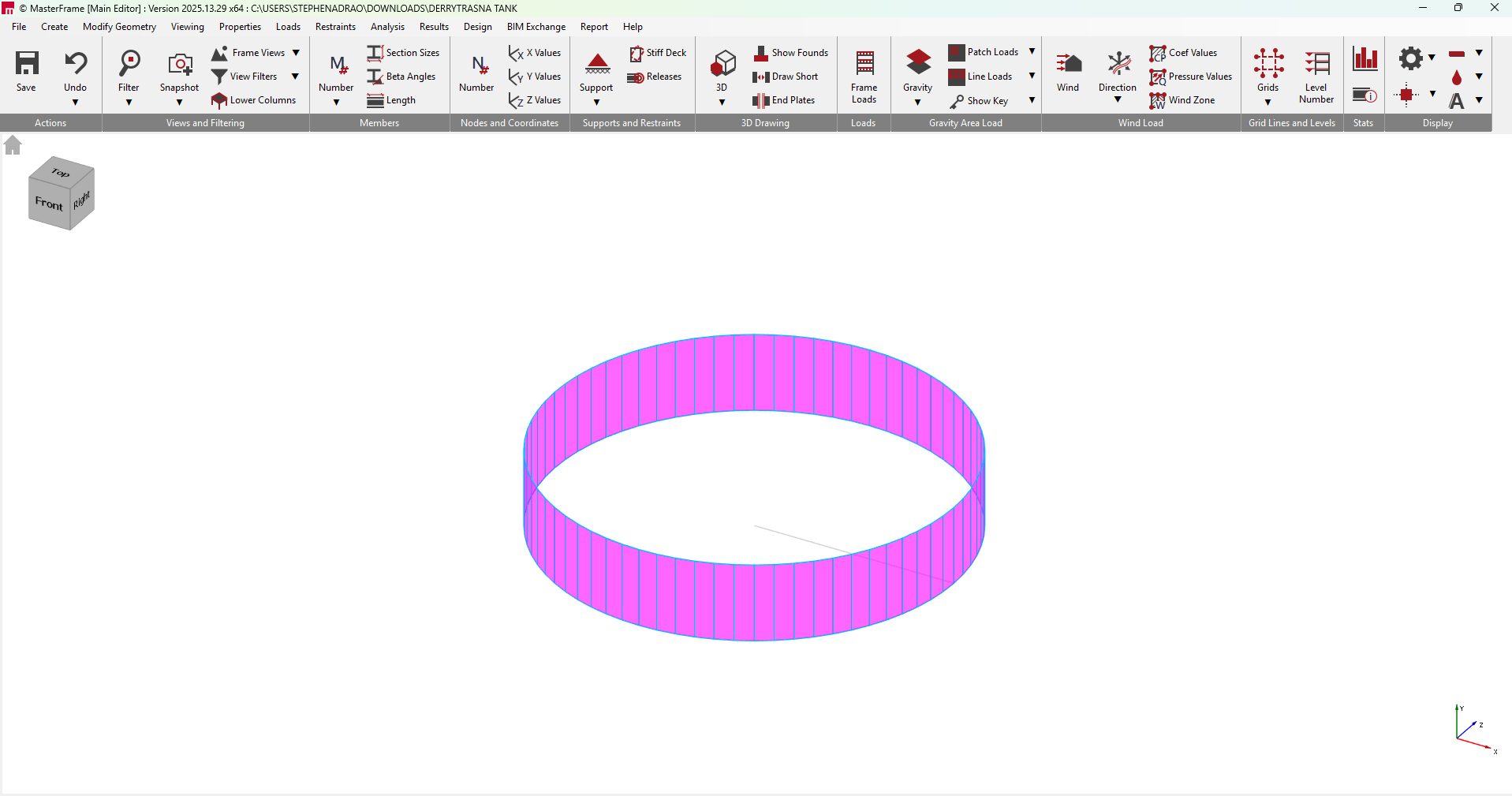
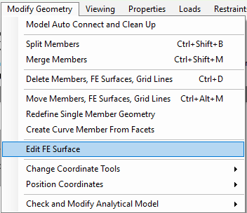
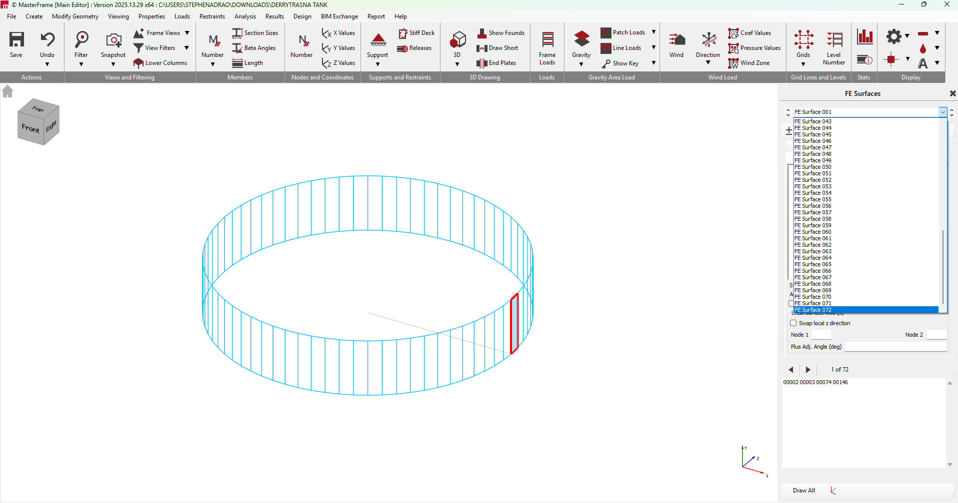
To check if you did this correctly, go to Modify Geometry and Edit FE Surface. You should have 72 FE Surfaces.
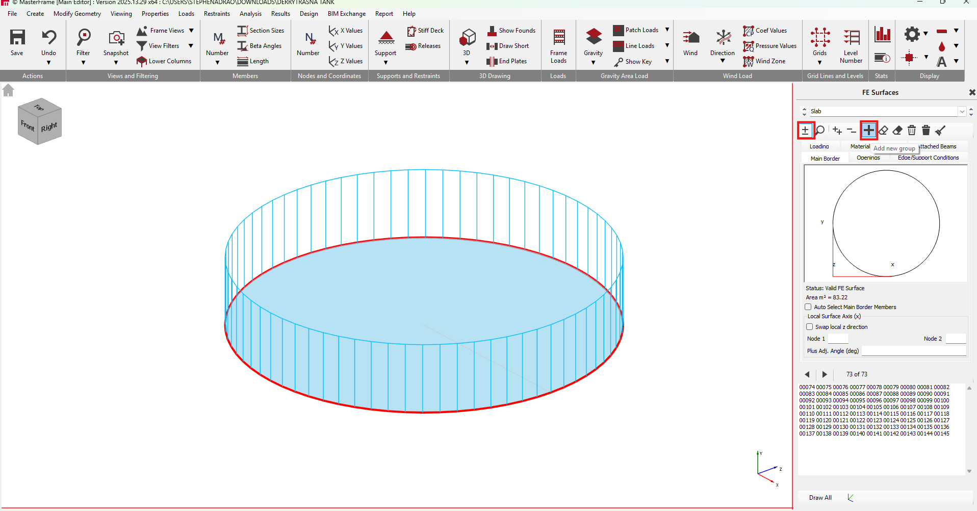
We will now create a new FE Surface calling it "Slab".
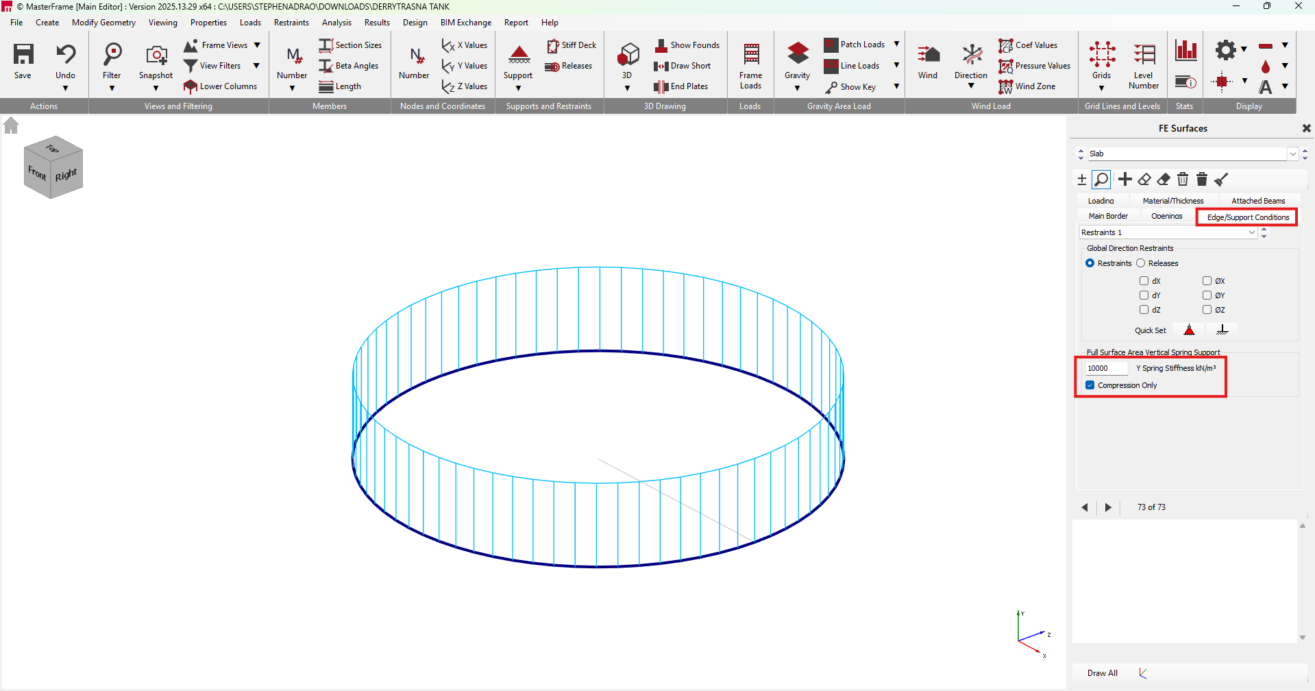
We are going to apply a Spring Stiffness of 10000kn/m3 at Compression Only.
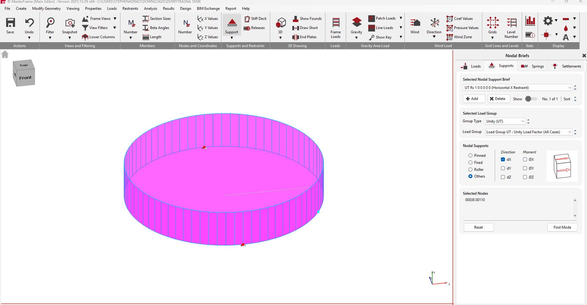
Applying Nodal Static Supports
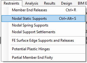
Go to the Restraints tab and click on Nodal Static Supports.
We will be applying nodal supports in the x direction, ensure that you are on to the Top View.

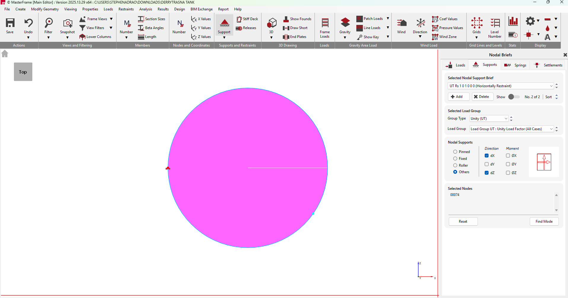
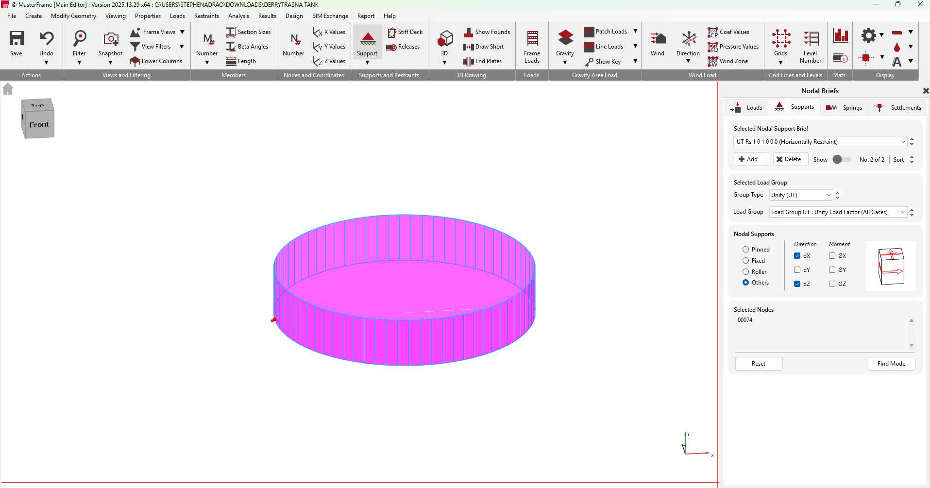
Now we will be applying nodal supports in the x and z direction. Click on Add and ensure you are on top view.
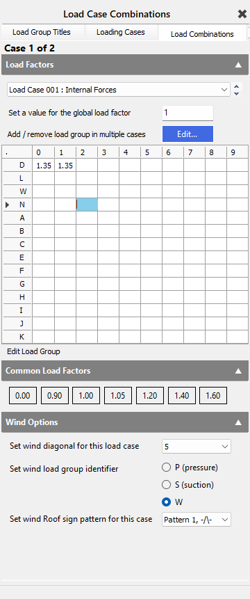
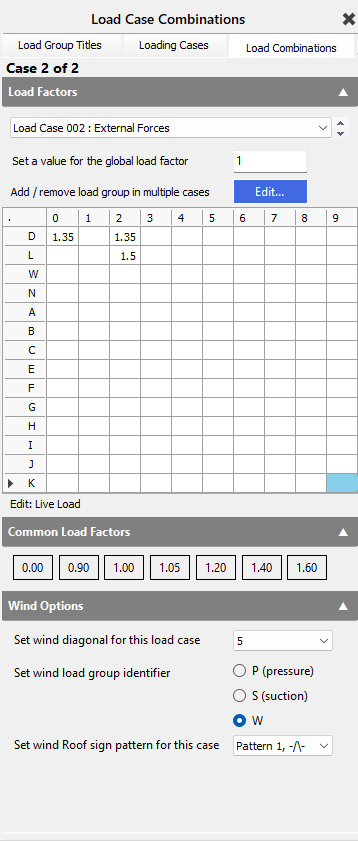
Load Cases and Global Editing
We will now generate load cases, go to Loads and then Load Cases.

Configure Load Cases: Set up titles for internal and external forces.
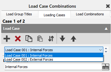
Go to the Load Combinations tab and set up the load combinations for the Internal and External Forces.
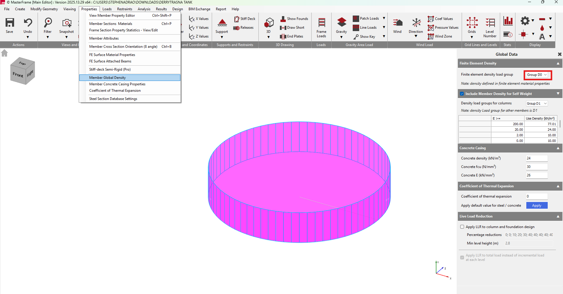
Go to the Properties tab and then Member Global Density. Change the Finite element density load group to D0.
Meshing with Stiff Regions
We are going to define our FE Surface Mesh. Go to Analysis, FE Surface Meshing and then Global Meshing Options.
Define Stiff Regions: At the intersections of walls and slabs, set up stiff regions (e.g., 0.225m) based on the thickness of the components.
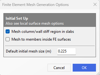
Prevent Stress Peaks: These regions are critical as they account for the physical thickness of the wall and slab, ensuring the analysis does not generate artificial stress peaks at the connection points.
Generate Global Mesh: Apply a global mesh, typically at a size matching the stiff region (e.g., 0.225).
Analysis and Results Review
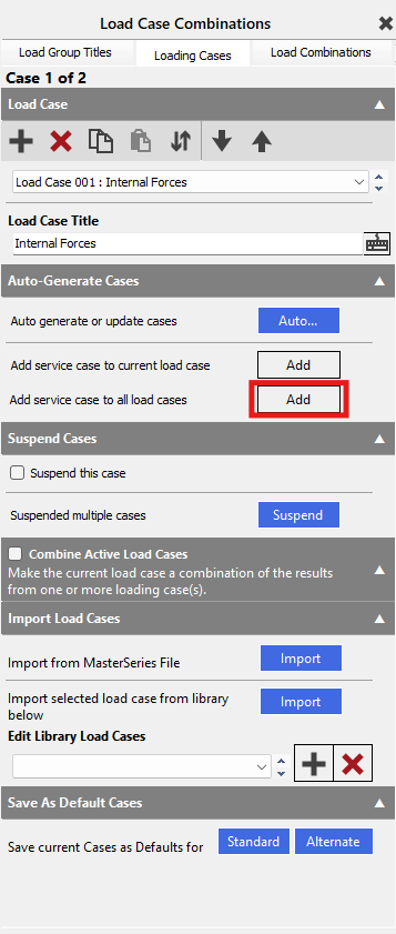
We are going to set up another load case by going to Loads and then Load Cases.
Add service case to all load cases.
It is always good practice to check the Frame Loads (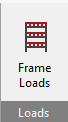 )
)
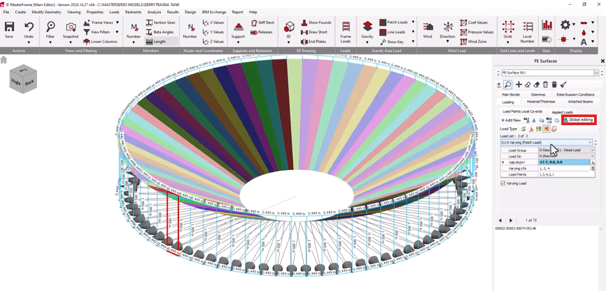
The model is currently back to front, to edit this, go to Modify Geometry and then Edit FE Surface.
Go to Loading and then click Global Editing.
Change the Vals Values for D1 to negative and then positive for D2.
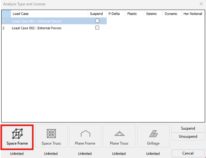
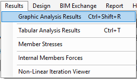
Run Analysis: Execute the graphical analysis for internal, external, and serviceability load cases.

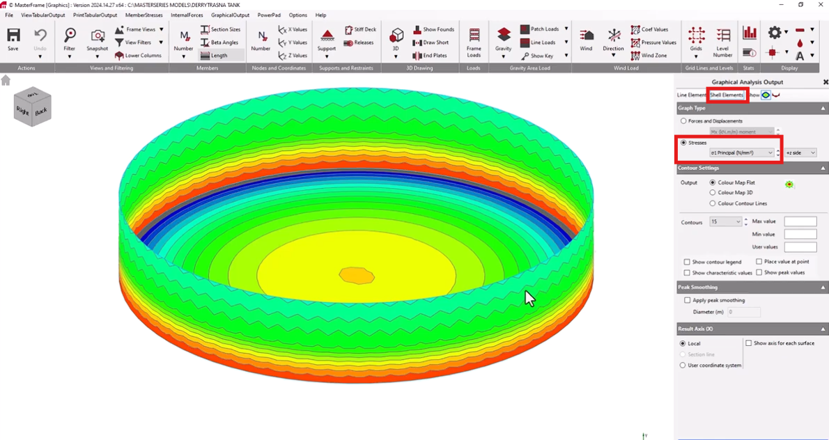
Go to Results and then Graphical Analysis Results.
Apply Surface Filters: To clearly inspect the performance of the walls, use the finite element surface filters to hide the slab. Go to View Filters, click on the Slab and then click Hide Selected FE Surfaces.
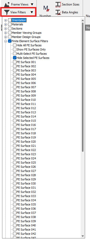
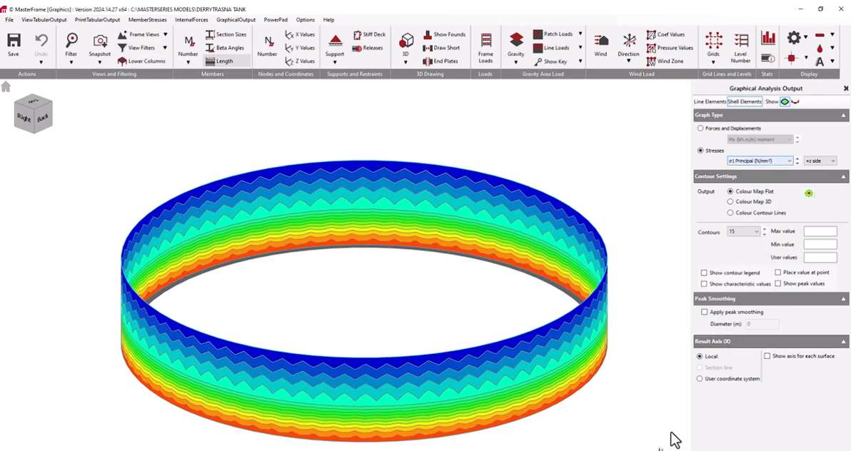
Inspect Stresses: Review the shell contour stresses to evaluate the structural integrity of the vertical walls without the visual interference of the base.